Modeling the Hemodynamic Response Function (HRF)
 HRF Models
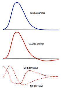
How, exactly should the shape of the HRF be determined for a given fMRI experiment? The term "canonical" HRF refers to the default shape selected by an investigator prior to data collection. Choices include a simple gamma function, a difference of two gamma functions (to allow for post-stimulus undershoot), Fourier basis sets, basis sets consisting of "plausible" HRF shapes, and finite impulse response functions. For improved accuracy the 1st and 2nd time derivatives of the HRF (commonly referred to as the "temporal" and "dispersion" derivatives respectively) may be added to the model. Use of these derivatives is equivalent to performing a second order Taylor series approximation of the HRF function. Including the 1st derivative allows timing of the peak response to be adjusted while the 2nd derivative allows the width of the HRF to vary.
To create a regressor, the chosen shape of the HRF is convolved with ("multiplied by") the experimental design. Nonlinear interactions among events that distort the expected HRF (such as two stimuli applied in a very short time frame where the total response may be less than the sum of the individual responses) may also be modeled using Volterra kernels or other methods.
To create a regressor, the chosen shape of the HRF is convolved with ("multiplied by") the experimental design. Nonlinear interactions among events that distort the expected HRF (such as two stimuli applied in a very short time frame where the total response may be less than the sum of the individual responses) may also be modeled using Volterra kernels or other methods.
Testing for Statistical Significance
The ultimate purpose of most fMRI experiments is to determine how the brain responds to various stimuli and conditions. For task-based fMRI studies the calculated amplitude vector β from GLM provides estimates (βi) of the relative weights ("importance") for each component (Xi) in the experimental design.
We begin with one of the simplest of all fMRI experiments: finger tapping. Here the subject alternately cycles between tapping her fingers and resting while BOLD responses over the entire brain are recorded. In this example the design matrix might contain just a single essential regressor denoted: X1 = "finger tapping". After data collection, GLM analysis produces an estimate (β1) of the amplitude response to finger tapping for each voxel. Voxels near the motor cortex would demonstrate strong responses with relatively large values of β1, while far-away voxels might only contain resting state "noise". So what criteria could we use to determine when we consider a voxel to be truly activated?
We begin with one of the simplest of all fMRI experiments: finger tapping. Here the subject alternately cycles between tapping her fingers and resting while BOLD responses over the entire brain are recorded. In this example the design matrix might contain just a single essential regressor denoted: X1 = "finger tapping". After data collection, GLM analysis produces an estimate (β1) of the amplitude response to finger tapping for each voxel. Voxels near the motor cortex would demonstrate strong responses with relatively large values of β1, while far-away voxels might only contain resting state "noise". So what criteria could we use to determine when we consider a voxel to be truly activated?
The formal/classical method of testing for statistical significance involves constructing a null hypothesis (Ho), which in this case might be written in words as "There is no net BOLD signal effect in a voxel during finger tapping compared to rest." In mathematical terms, this could be expressed as:
Ho: β1 = 0.
Ho: β1 = 0.
Typically null hypotheses are constructed in a negative/perverse way — i.e., that no fMRI effect is produced by a given event or action. In reality, however, we secretly wish to be surprised and find a result so unlikely to occur by chance that we can reject the null hypothesis.
By "statistically significant" we usually mean that the Type I (false positive) error of rejecting the null hypothesis is less than a certain arbitrary level of probability (p-value), perhaps p ≤ 0.05. In other words, we might call a result "significant" only when the probability of such an event happening by chance occurs less than 5% of the time.
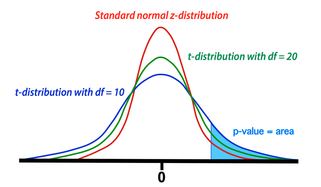
 Comparison between t- and z-distributions. As degrees of freedom (df) increase, the two converge.
The GLM calculation produces both an estimate for β1 and a standard deviation (SD) of this estimate. The SD depends on the sum of the mean squared errors as well as the structure and size of the design matrix (X). To test the null hypothesis, we form the test statistic T = β1/SD. Provided the assumptions of the GLM are maintained (i.e., errors are independent and Gaussian with mean zero), the statistic T follows a Student's t-distribution from which p-value percentiles can be determined. The precise shape of the t-distribution depends on the degrees of freedom (df), defined to be the number time points analyzed minus the number of independent regressors. The t-distribution is closely related to the Gaussian or standard normal (z-) distribution, converging to the latter as the df → ∞. In experiments with more than 100 observations, Z-values and percentiles are often reported instead of T-values, since the two are very close.
Multiple Regressors: Contrasts and F-tests
The finger-tapping example above contained only a single covariate of interest (X1 = "finger tapping") and its corresponding estimated amplitude (β1). Most interesting fMRI studies, however, include several regressors of interest. Let us consider a more complicated fMRI experiment wherein a subject is alternately shown red, blue, and green lights, alone or in combination. Three essential regressors of the design might be: X1 = "red light on", X2 = "blue light on", and X3 = "green light on". After data collection, the GLM would generate three amplitude estimates (β1, β2, and β3) corresponding to the three conditions that could be tested for statistical significance.
Multiple design variables allow combination effects to be investigated. For example, we might want to know whether a voxel was equally activated by the red light and blue light (β1= β2), or equivalently (β1 − β2 = 0). Or perhaps whether the average of red and blue illumination has the same effect as green illumination alone (½ [β1 + β2 ] = β3) , or equivalently (½β1 + ½β2 − β3 = 0).
These combinations are difficult to express in words, but can handily be represented in matrix form, multiplying each calculated amplitude vector β by a linear contrast vector cT. The two contrasts described above can be written as:
Even more complex hypothesis tests involving these multiple regressors could be imagined. For example, are the three means all equal to zero simultaneously? Or does a certain combination of lights lead to a significantly higher activity than another combination? In these cases, the contrast vector becomes a full matrix rather than a linear array of numbers, and the GLM procedure blossoms into a full analysis of variance (ANOVA). The applicable test statistic now becomes F instead of T, where F is formed by dividing the sum of squared residuals under a reduced model (without regressors) by the sum of squared residuals under the full model. Provided the usual GLM assumptions of identical and independent distribution of errors are preserved, the statistic F is distributed as according to the F-distribution which may used to test for statistical significance of hypotheses.
Autocorrelation of Data
One of the basic tenets of GLM — statistical independence of errors from point to point — is nearly always violated in an fMRI experiment. Functional MRI studies are not random collections of data but time series, with high values more likely to follow high values and low values more likely to follow low values. Quasi-periodic noise sources (such as cardiac and respiratory pulsations) also contribute to this phenomenon.
Fortunately, the presence of serial correlation does not affect estimates of the weighting parameters (βi). However, it does produce an underestimation of the error variance because the number of truly independent observations (the "effective" degrees of freedom, df) will be lower than the actual number of observations made. Thus t- or F-statistics, the shapes of whose distributions depend on df, will be artificially inflated, potentially resulting in elevated false positive rates and spurious inferences.
The most common method to control for autocorrelations is known as pre-whitening. The term "pre-whitening" refers to removing serial correlations in time series data so that its residuals have a more uniform distribution of frequencies similar to "white noise". Pre-whitening is performed through an iterative process. An initial GLM solution is first generated and the autocorrelation structure of the residuals is fit to a first or second order Auto-Regressive Model [AR(1) or AR(2)]. The original raw data is then adjusted by removing the estimated covariance structure and a second GLM performed on the "whitened" data.
Multi-Subject Analysis
Up to now we have discussed the GLM analysis of data from individual subjects only. To make fMRI conclusions more generalizable, individual results are often aggregated across multiple subjects or groups. Before statistical analysis is performed, however, the data from the multiple subjects must be warped into a common anatomic space (such as Talairach or MNI templates). This process is called normalization and has been described in a prior Q&A.
One of the earliest approaches for group analysis was simply to warp the data from all subjects into a normalized space and then concatenate it into one gigantic time series (as though the data were all recorded from a single "super" subject). This so-called fixed effects analysis has been largely abandoned because it does not adequately account for individual differences and cannot cleanly be used for making population inferences.
Multi-subject fMRI data is intrinsically hierarchical with at least two levels that must be considered: the individual and the group. A mixed-effect analysis is therefore more appropriate where errors are measured and considered both within and between subjects.
One method for doing this is a two-level GLM analysis. At the first level a standard GLM is performed separately for each subject. For the second level, however, only the βi values (not the full fMRI response data) are carried through where they become dependent variables. Second-level inferences can be difficult because the βi's are only estimates and their values are "contaminated" by variance from the first-level analysis. Several methods to handle this problem exist, one of the most popular being the restricted maximum likelihood technique using an expectation-maximization algorithm.
Advanced Discussion (show/hide)»
No supplementary material yet. Check back soon!
References
Related Questions
What causes magnetism?
What causes magnetism?


